4.5. Observing Tools

Observing Tools (OT) consist of components (observing panels, quick look data reduction, etc.) which astronomers and observatory staff use during runtime observing. For astronomers, operation also includes Phase I and Phase II proposal preparations that usually take place long before arriving at the telescope. The discussion below presents the System Level Requirements governing the OT, a description of the components that make up the OT, and how they are used to build the three most common observing applications of an observatory: the observing planning tools, the exposure time calculator, and an observing console.

Observing tools provide the following capabilities shown in the following Table, as derived from the System Level Requirements:

Title	Statement
Efficient Operations	Identify and define sequences for instruments, telescope, and science, operations to optimize on-sky observing efficiency, and to comply with GMT Efficiency Budget ( GMT-SE-REF-00593).
Telescope Operators, Instrument Specialists, and AO Specialists	Efficiently support the roles (operations, setup) of Telescope Operators, Instrument Specialists, and AO Specialists.
Quick Look	Provide software to facilitate near real-time assessment of data quality for each instrument.
Central Control Functions	Provide central control capabilities for every control subsystem.
Engineering Mode	Provide an engineering mode that allows low-level control of components and subsystems.
Observing Preparation Tools	Provide software tools to assist astronomers in the proposal preparation process.
Observatory Workflow Scheduling	Provide the capability to schedule and manage observatory workflows and tasks
Program Execution Planning	Provide the observatory staff software tools for advanced planning of observing programs.
Observing Program Definition	Provide software tools to assist astronomers in defining observing programs.
Observing Program Programs. Execution	Provide software tools to execute Observing
Calibration Efficiencies: AO, WFS, daytime, nighttime, routine, non-routine	Provide the capability to perform or support calibrations of all subsystems, instruments, AO, WFS, daytime, nighttime, routine, and non-routine calibrations within the time window specified in their respective requirements, and comply with GMT Efficiency Budget (GMT-SE-REF-00593).

4.5.1. Subsystem Description

The OT is composed of several components that can be invoked in different context during the observation life cycle. The OT components provide the following capabilities:

• Model Synthesis – Model synthesis consists of tools needed to generate models that feed into exposure time calculations for designing science observations, in all observing modes (GLAO, LTAO, and natural seeing), and with available instrument capabilities (direct imaging, long slit spectroscopy, IFU, multi-fiber / slit mask). Examples of existing tools include GALFIT [Peng10], Synphot (STScI), Pysynphot, GALAXEV [BrCh03], among many other packages and stellar libraries.
• Astronomy Source Catalog Database – The GMT astronomical sources catalog contains information (e.g., names, positions, and proper motions, radial velocities, redshifts, photometry) of stars, galaxies, asteroids, star clusters, gamma ray bursts, etc. The catalogs are merged from multiple sources. The star catalog database comes from Naval Observatory Merged Astrometric Dataset (NOMAD) that is currently composed of the Hipparcos, UCA2 (USNO CCD Astrograph Catalog), Tycho-2, and USNO-B catalogs. In all there are over 1 billion stars/galaxies. The system can incorporate new data sets as they become available (e.g., eventually the GAIA catalog should have gone through several releases) Information of new sources can be added to the astronomical catalog as they are discovered or assigned names by all-sky or targeted surveys. Information in the existing catalogs is updated based on a predefined schedule to remain current, especially for variable sources and sources with proper motion. Astronomers may wish to define specialized target lists where the objects do not exist in the object catalog maintained by the observatory. Such needs may arise when new objects are discovered (e.g., SNe, high redshift galaxies, GRB candidates), or in galaxy surveys where the galaxy names are assigned by the surveys, hence are not recognized by the IAU, or do not exist in any formal catalogs. Those objects may be stored for posterity, or temporarily within an user’s work area, or incorporated into the main system.
• Sky Calculator – The sky calculator computes the location of celestial objects at any given moment in time. The purpose of the sky calculator is to know how to register different coordinate systems (celestial, instrumental) into a common reference frame, allowing it to also compute the location and orientation of instrument footprints, slits, and fiber footprints, etc., that may then be used to produce graphical overlays during proposal and target-of-opportunity preparations. The same tool is used to predict where targets would be located in the instrument field of view during runtime operation. For non-sidereal targets, the sky calculator takes into account proper motion with time. Non-trivial, spherical geometry, sky and instrument coordinate transform calculations will be performed by SLALIB [Wall12b] and tcspk [Wall12a], using information from the pointing models. Many open source and Python-based tools are available for computing ephemerides, sky coordinate transformations, the World Coordinate System (WCS), including PyEphem, EphemPy, pywcs, etc.
• Overhead Time Calculator – The overhead time calculator estimates the overhead of certain observing component or sequences, such as telescope move, target acquisition, AO guide star selection and lock, detector readouts, etc. This calculator will be a custom tool built for GMT operations.
• Airmass Calculator – Given the RA and DEC of a list of objects, their proper motion, the time of the day and year, the location and altitude at the location of an observer, the airmass calculator computes the airmass of the object at a specified moment in time. Many existing airmass calculators are available on-line, including Skycalc (John Thorstensen), as well as subroutines in SLALIB.
• Asterism Facility – Given an image the asterism finder automatically determines asterisms from stars and galaxies, and then correlates them with positions of objects in the database to determine the celestial coordinate at the center of the image, as well as the coordinates of all the sources detected in the image. An example of an open-source astrometry tool is Astrometry.net [Lang10].
• Guide Star Finder – Given the position and color of a science target or telescope pointing, the guide star finder searches through GMTO star catalogs for bright stars that are suitable to be used as telescope and AO guide stars. A desirable feature is to allow users to update discoveries of binary stars in the searchable database. This algorithm also finds a suitable asterism for active optics guiding and wavefront corrections, as well as LTAO guide stars to achieve an appropriate Strehl requirement. The guide star finder takes into account restrictions due to vignetting by telescope optics, and for non-sidereal targets when the guide stars move into and out of the patrol range of the AGWS and NGS WFS.
• Object Observability – Object observability window calculator estimates when and for how long an object can be observed, restricted by criteria from the user, such as airmass, proximity to the moon, sky brightness (due to sunrise, sunset, and moon conditions), as well as proximity to AO guide stars for non-sidereal targets due to target motion, and other instrument restrictions, e.g., guide star vignetting. An example of a publicly available ephemeris tool for calculating sun, moon, and planet, positions is a Python tool called PyEphem.
• Positional Astronomy Facility – The positional astronomy facility is designed around SLALIB35, which performs spherical trigonometry, coordinate and time transformations that account for Earth axis precession, nutation, etc.
• Mosaic Creation – Given a set of images, the mosaic creation tool places those images into a common coordinate system using either WCS, asterisms in overlap regions, coordinate list of stars in images, etc. There are many generic software libraries, tools, and analysis environments, available for creating image mosaics, including those in IRAF, Pyraf, alipy, and Montage-Wrapper, which is a wrapper to the open source mosaic engine called Montage (http://montage.ipac.caltech.edu/).
• Model Database – To aid in exposure time calculations, the SWCS maintains a database of image and spectroscopy models that may be commonly used by observers. Image models include galaxies of different types, gravitational lenses, proto-stellar or proto-planetary discs, stars of different Strehl, etc. Spectroscopy models include galaxy, quasars, supernovae, stars, quasar absorption lines, etc. The model database can grow and be searched as users input their own models into the system.
• AO PSF Simulator – The AO PSF generator creates PSFs based on inputs specifying atmospheric seeing conditions, the brightness of an AO guide star, and the AO mode in use (natural seeing, LTAO, GLAO), at the location of the science target(s).
• Spectroscopy Mask Facility – The spectroscopy mask algorithm computes geometric transforms needed to map 2-D spectra onto detector focal planes from on-sky coordinates, accounting for parallactic angle. This is used help users visualize the placement of the spectrum / spectra on the detectors during observational planning phases.
• Observing Data Management – The observing data management tool is a database storing telescope proposals, observing programs, observing configurations, instrument definitions, observing blocks, observing sequences, etc., which are necessary to define observations and to facilitate their execution.

The design of the OT is based on a modular architecture that allows one to compose elementary components to implement the above capabilities. The observing tools are designed to be deployable in a cloud computing infrastructure. The core of the functionality is provided by components that run in a server. When an existing off-the-shelf package provides the required functionality, a thin wrapper allows its integration with the rest of the observatory software. The wrapper runs a server with a RESTful [FiTa02] and/or service oriented interface. In most cases a set of smart editors and view widgets deployed in a web browser would allow one to access the OT capabilities. These smart widgets can be instantiated in different contexts depending on the use case or workflow.

The OT design decouples the visualization rendering from the server component, which provides several benefits. It enables the use of server components for batch processing (e.g., as part of the scheduling process). It enables the deployment of server components in a cloud infrastructure that can be optimized to provide excellent performance. Lastly, it makes the Observing Tools globally available as part of the operational support infrastructure with an API that allows scripting. The last is what enables the workflows to be organized and distributed to teams observing together but potentially on different continents.

4.5.2. Application Examples

While the OT interfaces are either too numerous to present, are in conceptual stages, or will evolve over time as their operational use is better refined, this section illustrates examples and principles of those tools that will likely be heavily used. The following subsections serve to demonstrate how the OT basic components support three different contexts: an observation design tool, an exposure time calculator, and a real-time observing console.

Observation Design Tool (ODT)

The initial telescope proposal preparation as well as observation planning and design by astronomers will be based on a web-based interactive tool. The design tool serves several purposes:

1. To plan precise placements of science apertures, e.g., for creating mosaic observations, placing slit masks or fiber locations to avoid spectral overlaps
2. To locate stars for telescope guiding or for AO to achieve Strehl requirements for science, factoring in target airmass, distance and brightness of AO stars relative to science target
3. For non-sidereal targets, to optimize observing times and rotator orientation that maximize target and guide star tracking window

A concept of the functionalities is shown in Figure 4.8. The planning tool is often used during Phase I and Phase II proposal preparation. However, it may also be required during observing, in particular for targets of opportunity where prior information may not already exist, so that AO guide stars have to be selected on-the-fly. For non-sidereal targets, the ODT provides a real-time update of future observing windows based on guide star availability at any particular moment in time during the night. Several components of the ODT will thus be integrated directly into an observing console (see below) to facilitate that capability. The ODT will also fully integrate with a module that computes AO PSFs for the purpose of exposure time calculation, as discussed below. Note that with the GMT, the operational necessity of having multiple guide stars (4 for AGWS, and NGS for AO, etc.) may impose certain orientation constraints. Therefore the ODT is generally expected to be more widely used during observation than it has been in prior telescope designs, where it was primarily used during Phase I and Phase II of proposal preparations. For targets of opportunity observations, the ODT provides a seamless way to integrate capabilities to select guide stars and to estimate PSF Strehl on-the-fly given the concurrent runtime seeing and observing geometry.

The workflow of the ODT starts with a user selecting targets from astronomical source catalogs, which brings up a visualization display (e.g., Figure 4.8) showing the surrounding region. In this display, a user selects the observing mode (natural seeing, LTAO, GLAO), which uploads appropriate presets and parameter files for the user to specify. The user chooses a science instrument and its orientation to overlay the science target apertures. Based on known geometry between all the telescope instruments and sensors, the ODT automatically finds and selects the appropriate stars for guiding by querying the astronomical source catalog server, followed by a request to the sky calculator server to obtain aperture footprint coordinates for all the relevant instruments involved in acquisition, guiding, phasing, and science. One may choose to visualize the guide star selection, but doing so is generally optional and the process is transparent to the user if guide stars are available, unless it is necessary to fine-tune the selection (e.g., for non-sidereal targets).

With guide stars known a priori, this information would feed into the TCS to position the AGWS guide probes during telescope slewing – a process which is also transparent both to the user and the telescope operator. If no guide stars fall within the AGWS and/or OIWS FOV during observation planning, the software would alert the user to choose a different science position angle that is more feasible. In that situation the visualization display would show suitable guide stars so that users may easily judge the required rotator angle. Throughout this process, the sky calculator is responsible for knowing the relative positions of the various instrument footprints in the focal plane, and LGWS constellations, as shown in Figure 4.8

In most cases, guide star selections are intended to be automatic and transparent to users, except possibly for the AO NGS, which often need fine-tuning. For AO and non-sidereal observations, it is critical to select guide stars in Phase I of the proposal preparation stage to ensure technical feasibility even before arriving at Phase II. Observing non-sidereal targets may involve choosing multiple guide stars because the AGWS probes have to move relative to the science target during exposures. Sometimes it may be necessary to define different guide stars even within a single exposure. Based on known sky-projected motion of a non-sidereal target, the sky calculator would help by displaying its on-sky trajectory, finding guide stars that allow for the longest observing windows along that trajectory, and time-stamping locations (using LST) and airmass, to ensure that the proposed observing duration is attainable before arriving at the telescope.

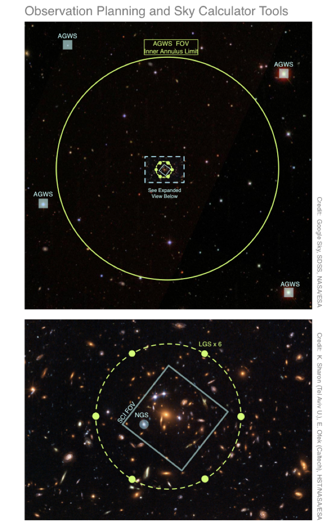
Fig. 4.8 Observation Planning and Sky Visualization / Calculator Tools (schematic). Observation planning and sky visualization / calculator tools helps one to find appropriate AGWS, GLAO, and OIWS guide stars, and helps to visualize the locations of science targets and instrument footprints relative to the guide stars. The LGS constellation has a diameter of 1 arcmin.

For AO observations, the ODT will estimate the performance of the AO system at the location of the science targets by using an AO PSF simulator module. Based on the geometry between the science target(s), the NGS, the LGS beacons, the demand (or current) seeing condition, airmass, etc., the simulator would provide a Strehl map around the science field. In addition, the PSF simulator would also produce PSF images at the location of the science targets for the purpose of the Exposure Time Calculator.

Exposure Time Calculator (ETC)

The ETC is one of the key tools for ensuring that the planned observations will produce scientifically useful data. Given information about the spectrum of a target, its geometry (point source, extended), flux (total or surface brightness), and some information about the detector (gain, pixel binning, background, etc.), traditional ETCs provide signal-to-noise (S/N) calculations for integrated flux or on per-pixel basis, and may output a spectrum for spectroscopy. While doing so may suffice for natural seeing observations (but often actually do not), the use of LTAO and NGSAO as primary modes of observing, and the high operation costs, demand substantially better tools to ensure realistic modeling predictions on which to base science justifications. This is especially crucial for studies of sharp features and extended sources whose sizes are near the seeing limit. In such cases, the value of S/N can vary dramatically depending on the profile shape and size of the object, the location where S/N is calculated, and the Strehl. The AO Strehl itself being dependent on a number of observational factors (distance and brightness from the NGS, seeing, etc.), and that Strehl may in the end not be the most useful number to use for extended sources, means that users will require a lot more guidance to help decide on technical feasibility. The GMT ETC, while providing the standard S/N summary, will also provide model data back to users for their own analysis. The model data will account for all known instrumental characteristics (readnoise, thermal background etc.), and other factors that affect AO observations based on observing configurations from the ODT. The purpose of the ETC is to make the creation of model simulations that are scientifically discriminating a transparent process for astronomers and observers.

Each instrument team is responsible for providing its own version of the ETC especially with regard to the noise property and sensitivity of the instruments. As the needs become warranted, the ETCs components provided by the instrument teams will be the starting basis to extend a modular model generation approach, both for imaging and spectroscopy (fiber, slits, IFS) observations. The components for the ETC are shown in Figure 4.9, consisting of:

1. A visualization display that allows for interactive creation and crosscut views of models
2. An image database or a generator based on GALFIT [Peng10] or equivalent tools as they become available
3. A spectrum generator or database
4. A noise simulator that takes into account all known sources
5. An AO PSF generator that accounts for the natural seeing, locations and brightnesses of the natural and laser guide stars relative to the science target of interest
6. Information regarding instruments: filter transmission curves, pixel size, binning factor, readout noise, gain, etc.

Users may also provide their own images and spectra to be used for calculations.

All the source codes for these components already exist and are freely available for reuse. In contrast to some of the previous ETCs, the GMT ETC would integrate seamlessly into the observation planning workflow to facilitate computation of PSF. Thus, exposure time calculation and observation planning need not be separate and independent steps, although each tool may be used independently, and outside of the other tool.

Model creation for imaging and spectroscopy ETC would both involve image generation (Figure 4.10), or the use of a pre-existing image, as the first step. The image is convolved with a PSF, created using an AO PSF simulator. If used with the observing planner, the observing configurations will propagate to the AO PSF simulator, to produce PSFs at target location(s) in the science FOV. Then, noise will be added to account for target brightness, exposure time, instrument readnoise, and thermal background.

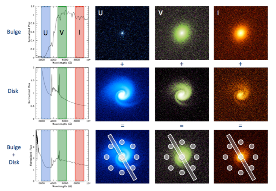
Fig. 4.9 Exposure Time Calculation of long slit, fiber, and integral field, spectroscopy to simulate resolved stellar populations study in a galaxy. Images are generated using a model image synthesizer, convolved with the PSF. The images are normalized at the desired wavelength slices given spectra produced by a spectrum synthesizer. Top row: Image simulation of a galaxy bulge in different wavelength slices (e.g., broadband U, V, I). Middle row: Image simulation of a galaxy disk in different wavelength slices. Bottom row: Combined Bulge and disk models. Detailed spectra can then be extracted in different apertures, slits, or maintained whole as a data cube, to be delivered back to astronomers for estimating signal-to-noise, or for feature extraction.

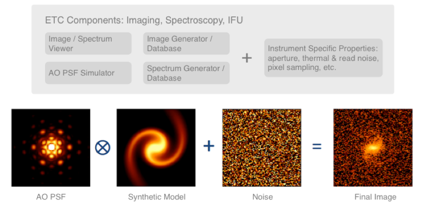
Fig. 4.10 Exposure Time Calculator basic model generation. The basic ETC components consist of a sophisticated PSF generator that accounts for observing mode and Strehl due to brightness and relative locations of guide stars; parallactic angle; image, spectrum, and noise, generators, that accounts for sky/thermal and instrument noise, and other instrument characteristics. In the image shown, a synthetic model is convolved with the AO PSF and added noise, to produce the final image.

Creating a spectroscopic model of an observation essentially uses the same image generation technique, but one also must account for spectral and spatial distortions, and mappings from the sky to the detector. The images are then normalized to object spectra at the appropriate wavelength slices shown in Figure 4.9. Like before, the model generator convolves all image slices with the PSF from the AO PSF generator then adds noise to the images. This outcome is a 3-D data cube (with two spatial [x, y] and a wavelength axes) that the user may retrieve and analyze. This technique allows one to create arbitrarily complex and realistic models where even the spectrum may vary spatially, such as for studying spatially resolved stellar population studies at high redshifts. As shown in Figure 4.9, the way to create such a model is to use different spectra for the different physical components: bulge (top row) and disk (bottom row), the net sum of which is shown in the bottom row. To obtain spectra for any aperture (fiber, long slit, masks), one would simply extract the data along the wavelength direction, as shown in Figure 4.9, bottom row. This enables users to have a more precise control, and more accurate determination of S/N, which properly account for all the known observing variables. User visualization and interfaces analogous to Figure 4.9 will permit users to operate the model creation at a high level, while hiding all the technical details regarding model generation so that they may focus on model design at a high and intuitive level for their science application.

Real-Time Observing Console (ROC)

Optimizing observing efficiency during runtime requires knowing the locations of the science targets in the sky (e.g., airmass to optimize image quality and observing duration), their proximity to the current pointing position (to minimize slew time, cable wraps), and environmental information such as cloud cover, wind speed and direction (that may preclude observation of certain targets in some directions). If the information needed to make informed decisions is distributed across different display panels, log sheets, etc., the task of manually optimizing an observing strategy can be more tedious than necessary, especially if target priorities change due to weather or other constraints. The purpose of the ROC is to integrate the following functionalities into a single display and user interface: target visualization, planning, selection, and environmental information (wind, clouds, etc.), for use during run-time observing. At a glance, observers and telescope operators should be able to have situational awareness of the most important and relevant information for observational planning. An example of the ROC is shown in the following Figure:

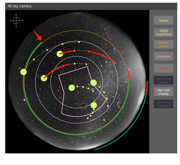
Fig. 4.11 On-the-fly observational planning and situation awareness tool (mockup). On-the-fly observational planning, target selection, and situation awareness (airmass, environmental information), are unified into a single visualization. Zenith is located at the center, and the 360 degrees horizon surrounds the outermost part of the view ports. The concentric circles represent airmass (or potentially elevation for AO operations), with solid orange circle being the elevation limit of the telescope, and dashed (inner) red circle being the zenith avoidance distance (exaggerated in figure). Dashed lines indicate the trajectories of the targets across the sky until astronomical twilight, and small circles along the trajectory indicate positions at hourly LST. Enclosure opening is represented in purple, shown with wind-shutter raised. The arrow near the edge of the portal represents wind speed and direction.

In the Figure above, the entire sky and the horizon are seen through a fish-eye display, with the zenith being located at the center of the panel, and the horizon located at the outer circumference. Concentric circles delineate the different airmasses, with high airmasses being larger circles. The elevation limit and zenith avoidance limits are shown as red circles in the visualization. The user will have control over which targets to show on the display via a menu that is user customizable; multiple menus can be used to group science targets and guide stars to reduce target crowding and confusion. Objects below the horizon will appear in the outskirts of the display, just outside the elevation limit circle. During the night, targets will move in arcs across the display, crossing through concentric circles of constant airmass. The arc trajectories of all the targets from current time to the end of the night are plotted in the display so as to inform their optimal visibility windows. Non-sidereal targets will have trajectories that appear and disappear depending on the visibility window due to guide star availability for a particular instrument orientation. Hourly locations of the targets from current time until astronomical twilight are shown as small circles along the trajectories. Placing a mouse cursor over the target trajectory would produce information regarding when the target would appear at that location, airmass, etc. Selecting a target in the display would allow an astronomer to send the target information to the TCS to slew the telescope, obtain more detailed information regarding the target, or to deselect the target. The ROC can also interact with the Scheduling System to instantaneously visualize the sky location of the targets during queue planning, as the weights are changed.

Environmental information is also provided in the same visualization display that may be turned on/off. If cloud information is available, via either the weather service or an all-sky fish-eye camera located near the site, then it may be rendered as a superposition in the fish-eye display (Figure 4.11). This would provide observers more educated ways to “shoot between the clouds” with a higher chance of success. Wind speed and direction are represented as arrows along the periphery of the display. The length and color of the arrows indicate wind speed, whereas the location along the periphery indicates incoming direction.